How it all started

Remember color-by-number from childhood? Some kids hated those. Me, I had my mother make regular pictures into color-by-number, now I knew exactly what to do! Fast forward a few years. “Pick a topic for your paper…”. That’s the hardest part, then to make it long enough… I would rather prove a theorem, thank you.

Fast forward many more years; I have forgotten almost everything about proving theorems. Hence, I am studying Data Science at Lambda School. It’s time to begin my Unit 2 Build Project. “Pick a data set…” Ugh, the worst part. I found this data set on Kaggle, TVS Loan Default, it seemed tidy and was brand new. I was so busy learning the mechanics from my lessons, I didn’t notice a problem. Little did I know, highly imbalanced data isn’t a great choice for a beginner. Trying to find a way to distinguish a tiny amount of data from all of the rest proved to be tricky. I learned about a new technique. Soon everything was going swimmingly. Then, the weekend before the project was due I happened upon a bit of information that set off that little niggling feeling… Sure enough, I had misunderstood how to apply the new technique. What I thought was working well was hardly working at all…

The Project

The Data

TVS is a lending institution which provides both secured and unsecured loans. A secured loan has something which can be repossessed if a customer defaults, for example: a two-wheeled vehicle. A personal loan is an example of an unsecured loan, if the customer fails to pay, the money is lost.

The data set was comprised of information on TVS customers who have already taken out a loan for a two-wheeled vehicle and would like to take out a personal loan as well. Around 2% of TVS borrowers default on their vehicle loans. If TVS can predict who will default on one loan, they will know not to approve another.

There is no data available about the people whose loan applications were denied. Hence, defaulters cannot be compared to the denied clients to find similarities. All of the clients have already passed through the TVS loan approval process.

Initially there were about 120,000 clients listed in my data set, with 32 possible pieces of non-identifying information about each one. This information is referred to as features or columns. Both clients and features with too many holes, that is missing information, had to be dropped. Several other columns containing details gathered after the loan was granted needed to be removed. Now there were about 85,000 clients and 11 columns of information. Defaulters made up just 2.18% of the client list. A balanced dataset would have about 50% defaulters.

Creating Models

Now it was time to begin creating a model to detect defaulters. Models are created by splitting the data into three groups. Training data, the largest group is used to create the actual model. Two other smaller groups of data are set aside. Validation data is used for practicing, how does the model perform? Testing data is saved for last and is used to verify performance.

The baselines for all of my basic models were abismal at 0.0%. None of the models identified a single defaulter!

Downsampling

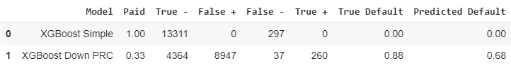
I tried two techniques for balancing the data. Downsampling was done by cutting down list of the non-defaulters to approximately the same number as defaulters. Downsampling generated my best gradient boosting model. The resulting baseline for defaulters was 89%, however it also predicted that 68% of all clients were defaulters.

Gradient Boosting Model

SMOTE

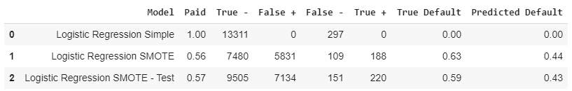
Synthetic Minority Oversampling Technique, works the opposite of downsampling. SMOTE was used to create a fictional population of defaulters to balance out the non-defaulters. It sounds a little fanciful, but is proven to be legitimate in the world of data science. Using SMOTE with a linear regression model gave my best results. On the test data the baseline for defaulters was 59%, with 43% of clients overall labeled as defaulters.

Logistic Regression Model

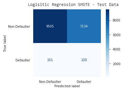
Here’s an easier way to look at the information for my best model. The top row represents non-defaulters; those predicted correctly are on the left. The bottom row represents defaulters, those predicted correctly are on the right. The opposite diagonal contains all of the incorrect predictions.

Visual Matrix

A third model

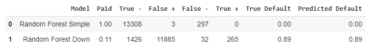
I also created a Random Forest model, it performed well before I discovered my error. The mistake was that I had downsampled all three data groups, the correct method was to downsample (or SMOTE) only the training group. Using data in the correct configuration this models best version found 89% of the defaulters. Unfortunately it also predicted that 89% of all clients were defaulters!

Random Forest Model

Let’s Pretend

Let’s pretend for a moment that Random Forest model I generated was actually fantastic. TVS considers adopting my model, but the bankers need more information about why clients are predicted to default.

“The mysterious black box predicts that this client will default” isn’t going to work. However, there is a helpful way to illustrate how the model selected it’s results. This Shapley, not shapely, plot will help the banker understand which factors are most important.

Shapley Graph

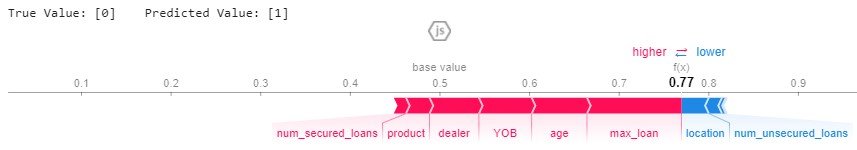
Client Information

This client is young, has no secured loans with TVS, and wants to purchase a trailer for $39,000, all of these factors are going against him. His location and not already having an unsecured loan with TVS are in his favor.

The Conclusion

Unless TVS wants to sell a large percentage of their personal loans to another lender, my models are not particularly useful. However, school projects are intended to be learning experiences, so the most important goal was achieved.

Other useful information

Find my raw data here: TVS

Take a peek at my code here: Build_Notebook

Photo by Sonya Lynne on Unsplash

The Teacher was considered wise…studying and classifying…

Ecclesiastes 12:9 paraphrase